Here is the equation for the 2-D receptive field:

w     = the radius of the receptive field
s_e         = the standard deviation of the excitatory center
s_i          = the standard deviation of the inhibitory surround
i,j          = the position within the receptive field of the receptor

In this instantiation of the model, the width is set to 3*s_i, or three times the standard deviation of the surround which is inhibitory in this cell.  The one odd value from the standard DOG equation is the ratio or weight at the beginning of the excitatory receptive field.  This was necessary to balance out the increased surround area going from the 1 dimensional to the 2 dimensional version of the model.  By adding the second dimension, the surround grows at a greater rate since it is larger (area of a circle is Pr²).  A linear adjustment is all that is necessary because they were balanced in one dimension and only need to compensate for the second dimension.  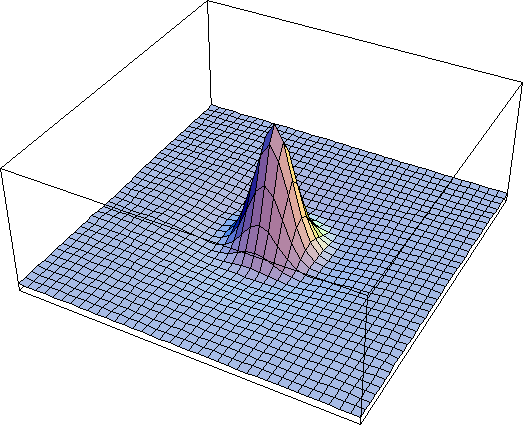The resulting map of sensitivity is shown below.

The inhibitory region is not as visible due the the greater amplitude of the central region.

This page illustrates how the model works in a very basic way.