If you need a review of receptive fields, I recommend this review (Krantz, 1994) and this powerpoint illustration (Krantz, 1998).

The two types of receptive fields discovered by Enroth-Cugell and Robson (1966, 1984) were called by them, X and Y.  Both had the center surround properties found by Kuffler (1953) in his classic paper that introduced the idea of receptive fields to us.  However, these X and Y cells differed in some important ways.  Below is a general table that specified their response properties.

The idea of a fairly stable response pattern by X cells is that the firing rate for the cell is fairly constant during the whole duration of the stimulus.  If the cell is firing 100 times a second when the stimulus comes on, it stays that same firing rate throughout the duration of the stimulus.  On the other hand, Y cells show an of-off firing rate.  They fire a burst when the stimulus is turned on and then return to the baseline firing rate.  Another burst is often seen in these sells when the stimulus is turned off, thus the on-off label (See the figure below).  This transient pattern of responses have often been taken as a good source of the signal for motion coming out of the retina, just see any introductory sensation and perception text book (Coren, Ward, & Enns, 1999).  More sophisticated models of the visual system make the same conclusion (e.g. Zeki, 1993).

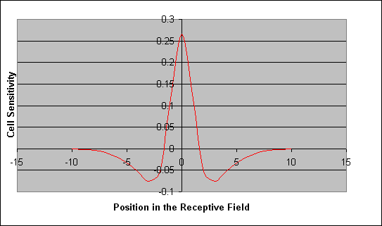
Ganglion Receptive Fields are DOGs

An important element of the work by Enroth-Cugell & Robson (1984) is their work to describe the receptive fields as the difference of two gaussians.  These functions are called DOGs for Difference Of Gaussians.  The figures below illustrate this concept. The first figure shows the theoretical distribution of excitation and inhibition across the receptive field.  Every point that falls on the receptive field stimulates both inhibition and excitation.  The relative amount of excitation and inhibition are controlled by the standard deviation of the their respective distributions and the position in the receptive field.

The resulting output is simply the sum of these two opposing effects.  The figure below shows the result of this operation.   Now recall this is a one dimensional representation of a two dimensional receptive field, if you spin this patter around the center of the two gaussians you will get the classic center-surround receptive field.

This receptive field is an on-center receptive field.  That is light in the middle section stimulates the cell and increases its firing rate.  Light in the surround inhibits the cell.  To get an off-center cell simply make the standard deviation for the inhibition smaller than the standard deviation for the excitation.

Below is a 2 dimensional representation of the this receptive field with the height of the surface representing the magnitude and sign of the response.